Treating pixels as vectors

It is common knowledge that images can be thought of as a 2-dimensional collection of pixel values. But, has anyone ever told you how to think of pixel values?

A friend once told me:

You can think of pixel values as vectors, and in the math. vectors have magnitude and direction.

The thought that you could treat pixel values as vectors was really interesting. I began to think of all of the crazy things you can do with vectors, and how interesting that would be to do with pixels.

Note

In our case we will be working with Red, Green and Blue (RGB) pixels. There are a wide variety of pixel formats out there, but we’re just going to work with RGB.

In this tutorial we will be thinking of RGB pixels as XYZ cartesias coordinates. This means that we can perform the same 3D math on pixels the is common with 3D vectors. However, instead of manipulating an XYZ coordinate in 3D space, we are manipulating an RGB pixel in color-space!

This was a mind-bending thought experiment, and I hope you’ll enjoy it.

Initial imports

from pathlib import Path

import matplotlib.pyplot as plt
import numpy as np
import PIL.Image
from scipy.spatial.transform import Rotation

Reading an image as a numpy array

Here, we will use matplotlib’s image functionality since this offers more than what we need.

Matplotlib will convert our pixel values to float32 with values ranging from [0.0 … 1.0]. This is perfect for our case. Typically, images are stored in uint8 with values ranging form [0 … 255]. Since we are trying to do 3D math on our pixels, it is easier to use float values.

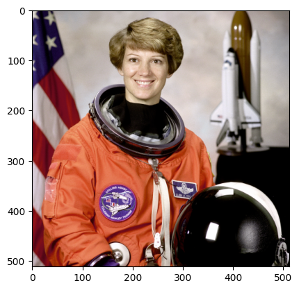
img_path = Path("../res/astronaut.png")
img = np.array(PIL.Image.open(img_path)) / 256.0
plt.imshow(img)
plt.show()

Since we’ll be doing some 3D math on our pixels, we may end up with values outside of the range [0…1], so lets’s create a simple plotting function to correct any of this.

def plot_img(ax: plt.Axes, title: str, img: np.ndarray) -> None:
    """Show an image.

    Pixel values are clipped to the range [0...1].
    """
    ax.imshow(np.clip(img, 0.0, 1.0))
    ax.set_title(title)


def plot_histogram(ax: plt.Axes, title: str, img: np.ndarray):
    color_index_map = {"red": 0, "green": 1, "blue": 2}

    def _plot_hist(img, color):
        hist, bins = np.histogram(img, bins=128)
        ax.plot(bins[:-1], hist, color=color)

    for color, index in color_index_map.items():
        _plot_hist(img[:, :, index], color)

    ax.set_title(title)
    ax.set_xlabel("pixel value")
    ax.set_ylabel("occurence")
    ax.set_ylim((0, 7000))


def plot(operation):
    def do_operation_and_plot(img, *args, **kwargs):
        img_op = operation(img, *args, **kwargs)

        xmin = np.min([img, img_op])
        xmax = np.max([img, img_op])

        fig = plt.figure(constrained_layout=True)
        gs = plt.GridSpec(2, 2, figure=fig)

        for i, (img_array, title) in enumerate(
            [
                (img, "Orig"),
                (img_op, "New"),
            ]
        ):
            ax_img = fig.add_subplot(gs[0, i])
            plot_img(ax_img, f"{title} Image", img_array)

            ax_plot = fig.add_subplot(gs[1, i])
            plot_histogram(ax_plot, f"{title} Hist", img_array)
            ax_plot.set_xlim((xmin, xmax))

        plt.show()

    return do_operation_and_plot

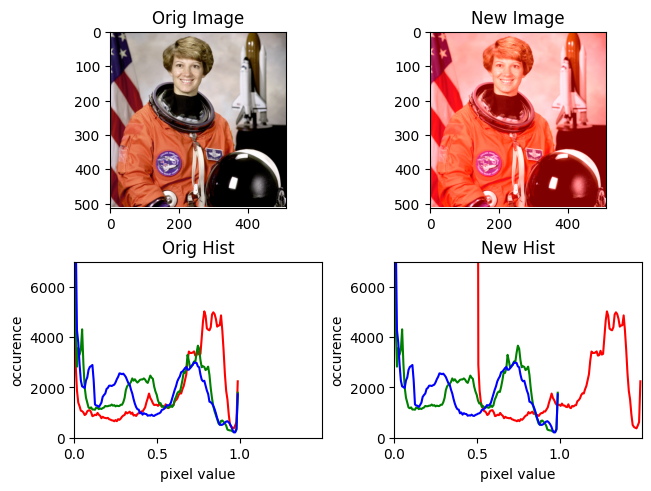
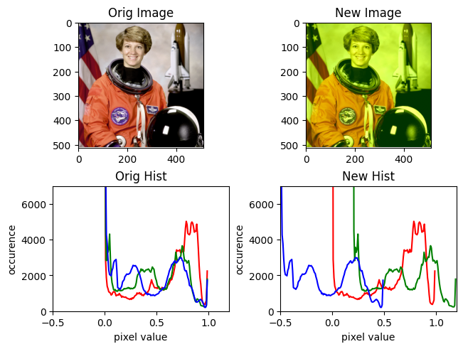
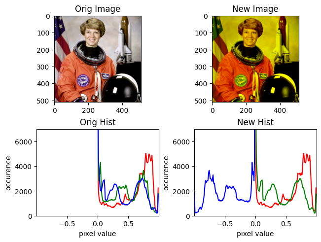
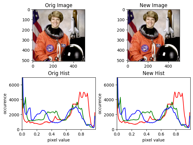
Translations

Think of translations like sliding the values higher or lower. We can translate only one color, or we can translate multiple colors at the same time.

@plot
def translate(img, *, r=0.0, g=0.0, b=0.0):
    return img + np.array([r, g, b])

translate(img, r=0.5)

translate(img, b=-0.5, g=0.2)

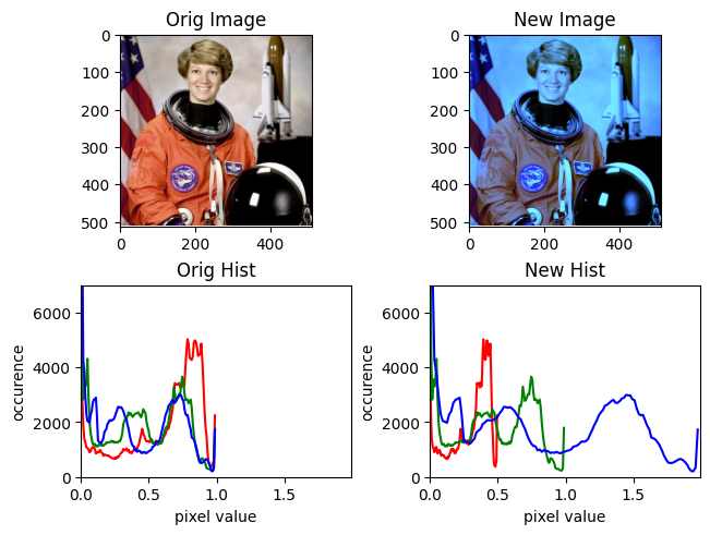
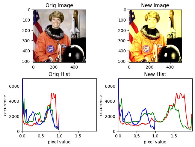
Scaling

Scaling is simply multiplying a color by a factor.

@plot
def scale(img, *, r=1.0, g=1.0, b=1.0):
    return img * np.array([r, g, b])

scale(img, r=0.5, b=2.0)

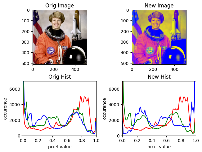
Rotation

Rotations are a bit more complicated to think about. In a cartesian coordinate system all axes are orthogonal, meaning that they are each perpendicular to one another. When we rotate a vector, we have to define two things:

1. A vector around which we rotate

• We can simply rotate around specific axes

2. A point around which rotate

• Typically the origin

Remember that RGB corrpesponds to XYZ, so rotating about X is the same as rotating about Red.

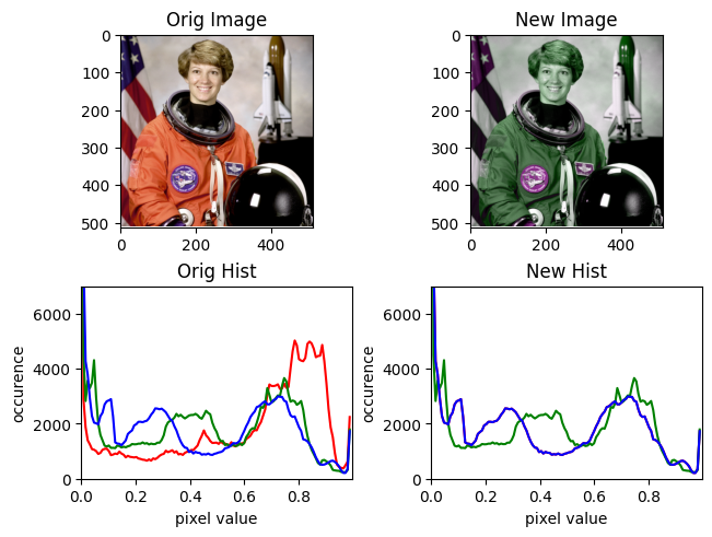
For example, when we rotate 90 degrees around Red axis, about the origin, then Green goes into the Blue axis, and Blue goes into the negative Green axis.

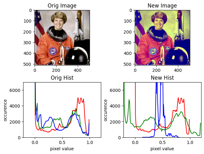
With 3D points, rotating about the origin makes sense, but for colors, rotating about the origin (0, 0, 0) is akin to rotating about black… it makes more sense to rotate about (0.5, 0.5, 0.5) which is akin to rotating about grey.

@plot
def rotate(img, rotation: Rotation, origin=[0.5, 0.5, 0.5]):
    img_rot = np.matmul((img - origin), rotation.as_matrix()) + origin
    return img_rot

rot = Rotation.from_euler("x", 90, degrees=True)

Here’s what it looks like rotating about black:

rotate(img, rot, origin=[0, 0, 0])

Here’s what it looks like rotated about gray.

rotate(img, rot)

rotate(
    img,
    Rotation.from_euler(
        "x",
        45,
        degrees=True,
    ),
)

rotate(
    img,
    Rotation.from_euler(
        "z",
        90,
        degrees=True,
    ),
    origin=[0.5, 0.5, 0.5],
)

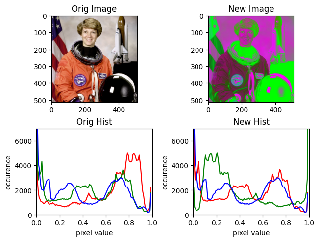
Custom Transformation Matrices

Now I’m just going a little too far, but you can actually define custom transformation matrices. I don’t really know what I’m doing here, so I will refer to these custom matrices as crazy matrices.

The way the function below crazy_mat works is that you define where you want your new RGB axes to go, and then it creates the crazy matrix for you.

def crazy_mat(
    r=[1, 0, 0],
    g=[0, 1, 0],
    b=[0, 0, 1],
):
    return np.array([r, g, b]).T


@plot
def do_crazy(img, **kwargs):
    return np.matmul(img[:, :, 0:3], crazy_mat(**kwargs))

The default crazy matrix is just the idendity matrix, and nothing will happen.

do_crazy(img)

Now, let’s say we want to swap our Red and Green axes while leaving our Blue axis alone. We can probably achive this by performing a series of rotations, but it’s much easier to define a custom transformation matrix.

do_crazy(img, r=[0, 1, 0], g=[1, 0, 0])

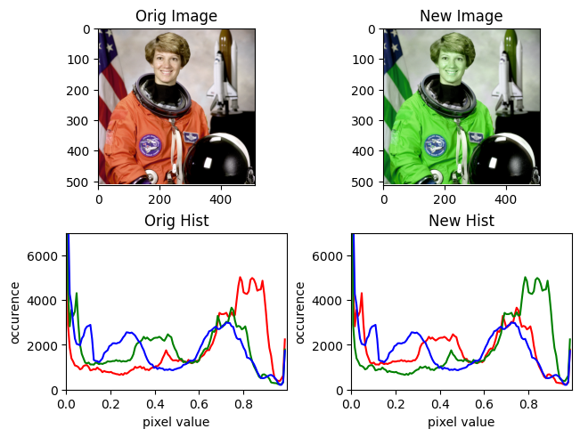
You see how this did exactly what we said! The Red and Green swapped places!

We can use this handy transformation matrix to even perform scaling!

do_crazy(img, r=[2, 0, 0], g=[0, 2, 0])

Which is the same as if we just used our previous scaling function.

scale(img, r=2, g=2)

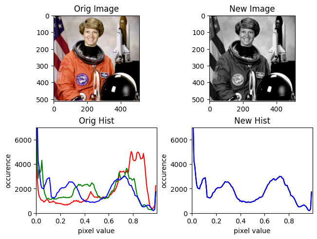
We can even collapse colors into a single dimension, making the color grayscale. Let’s collapse both red and green into the blue dimension.

do_crazy(img, r=[0, 0, 1], g=[0, 0, 1])

Or collapse only one color into another dimension. Let’s collapse red into blue.

do_crazy(img, r=[0, 0, 1])

Magnitude

We haven’t yet discussed getting the magnitude of a vector. This is its length, or distance from the origin.

For colors, the origin is black, so its distance from black can be thought of as its brightness.

def compute_magnitude(img):
    img_mag = np.empty_like(img)
    mags = np.linalg.norm(img, axis=2)
    for i in range(3):
        img_mag[:, :, i] = mags
    return img_mag


@plot
def magnitude(img):
    return compute_magnitude(img)


magnitude(img)

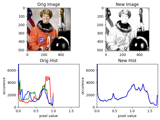
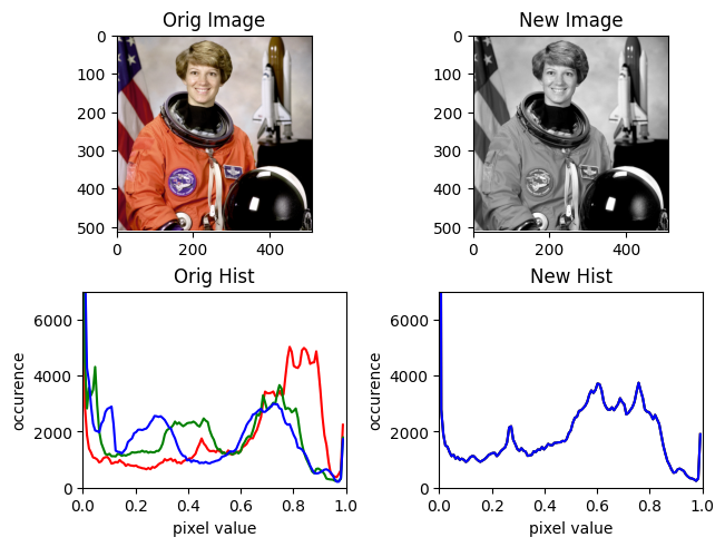
You see that some magnitudes are greater than 1.0. We can normalize those.

def compute_normalized_magnitude(img):
    mag = compute_magnitude(img)
    return mag / np.max(mag)


@plot
def normalized_magnitude(img):
    return compute_normalized_magnitude(img)


normalized_magnitude(img)

Direction

So, what can we do with direction? Here’s an idea: The dot-product of two vectors returns the angle between those vectors.

Anyway, if I have time to do a demo I will, but this article is getting pretty long, so it’s probably time to wrap it up.