xarray for modeling and simulation

First of all, xarray is a wonderful tool for creating - and interacting with - labeled multidimensional data. I turn to xarray any time I have multidimensional data.

The purpose of this tutorial is to (hopefully) show you that performing computations using xarray is easy. xarray’s API makes your multidimensional computations much more expressive, and easier to understand!

Defining the problem

Imagine we’re working on a modeling and simulation project where we want to model the trajectory of a projectile in 3D space. Our projectile has onboard sensors such as accelerometers, thermometers, etc. We want to simulate this sensor data, and then use that data to compute useful things such the position of our projectile is in 3D space.

Simple enough, right?

Simulating sensor data

Of course, we don’t have a real projectile with sensors. We will need to model some sensor data.

Let’s keep things simple for now. Let’s focus only on modeling the projectile’s path over time.

To model the projectile’s path we’ll have to model some accelerometer data that informs us of the projectile’s x- y- and z-acceleration over time.

import matplotlib.pyplot as plt
import numpy as np
import xarray as xr
from IPython.display import Math


def gen_linspace_values(start, stop, n):
    """Generate linearly spaced values, then add same noise."""
    values, step = np.linspace(start, stop, n, retstep=True)
    noise = step / 5
    noise_values = np.random.default_rng().normal(0.0, noise, size=values.shape)
    values = values + noise_values
    return values


def gen_centered_values(center, shape, noise):
    """Create values distributed about a center, then add some noise."""
    noise_values = np.random.default_rng().normal(0, noise, size=shape)
    return np.array(center) + noise_values

Time

Time will be stored in an xarray.DataArray, not a numpy.ndarray! This is because we can store so much more relevant info in an xarray.DataArray.

Think of an xarray.DataArray like a numpy.ndarray. DataArrays simply extend the capability of ndarrays.

Let’s also add some noise to the time measurements.

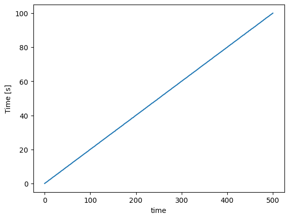
time = xr.DataArray(
    gen_linspace_values(0, 100, 501),
    dims=("time"),
    attrs={"units": "s", "long_name": "Time"},
)
time.plot()
plt.show()

X- Y- and Z- axes

We are dealing with 3D coordinates. It may seem trivial to define this data structure, but believe me, it makes things much more expressive and clear.

axis = xr.DataArray(
    ["x", "y", "z"],
    dims=("ax"),
    attrs={
        "long_name": "Axis",
    },
)
axis

<xarray.DataArray (ax: 3)>
array(['x', 'y', 'z'], dtype='<U1')
Dimensions without coordinates: ax
Attributes:
    long_name:  Axis

xarray.DataArray

• ax: 3

• 'x' 'y' 'z'

  array(['x', 'y', 'z'], dtype='<U1')

• Coordinates: (0)
• Indexes: (0)
• Attributes: (1)

  long_name :

  Axis

Acceleration

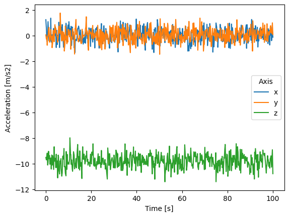
Let’s keep this simulation as simple as possible. Let’s assume that the only force acting on our projectile is gravity (acceleration of 9.81 m/s^2), and that gravity acts in the z-direction. The acceleration in both the x- and y- directions is zero.

Let’s go ahead and simulate some acceleration sensor data. acceleration data with some noise.

acceleration = xr.DataArray(
    gen_centered_values(
        [0.0, 0.0, -9.81],
        (len(time), len(axis)),
        0.5,
    ),
    coords=[time, axis],
    attrs={"long_name": "Acceleration", "units": "m/s2"},
)

acceleration.plot(hue="ax")
plt.show()

Our simulation object

So, we created the minimal amount of data: time and acceleration! Let’s bundle this data into our simulation object.

Our simulation will be an xarray.Dataset. Think of a Dataset like a collection of DataArrays.

simulation = xr.Dataset(
    {
        "time": time,
        "ax": axis,
        "acceleration": acceleration,
    }
)

Computations

Okay, we’ve created some data. Now let’s start getting to work! This is the part where we want to take advantage of some of xarrays functionality to make our computations more expressive!

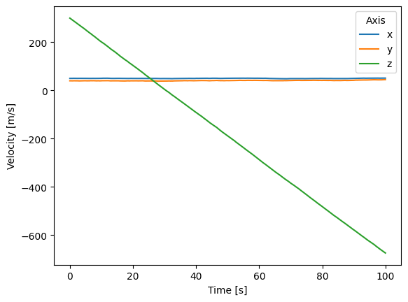
Velocity

First of all, I’m no mathematician or physicist, so my explanations may not be that great…

The equation for final velocity, given an initial velocity, constant acceleration and a time is:

Math("v_f = v_i + at")

\[\displaystyle v_f = v_i + at\]

In our case, we have multiple acceleration recordings, each with its own time stamp. So, we need to compute the change in time between each of the time stamp.

Our velocity at any point in time is then equal to the acceleration at that time, multiplied by how much time has passed since the previous recording, plus the velocity at the previous recording.

So, we need to decide an initial velocity. Let’s set it to some arbitrary value in order to keep things interesting.

initial_velocity = np.array([50.0, 40.0, 300.0])

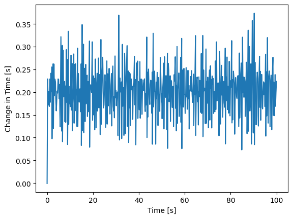
Now we need delta time. xarray has a very useful diff() function for computing exactly this, but we will use numpy.diff instead. See this Stack Overflow article for a small explanation as to why.

dt_values = np.diff(simulation.time, prepend=0)

simulation["dt"] = xr.DataArray(
    dt_values,
    coords=[simulation.time],
    attrs={"units": "s", "long_name": "Change in Time"},
    name="delta_time",
)
simulation.dt.plot()
plt.show()

simulation["velocity"] = (
    simulation.dt * simulation.acceleration
).cumsum() + initial_velocity

simulation.velocity.attrs["long_name"] = "Velocity"
simulation.velocity.attrs["units"] = "m/s"

simulation.velocity.plot(hue="ax")
plt.show()

Position

We can do nearly the exact same thing to compute the projectile’s position at every time stamp.

initial_position = np.array([0.0, 40.0, 10.0])

simulation["position"] = (
    simulation.dt * simulation.velocity
).cumsum() + initial_position

simulation.position.attrs["long_name"] = "Position"
simulation.position.attrs["units"] = "m"

simulation.position.plot(hue="ax")
plt.show()

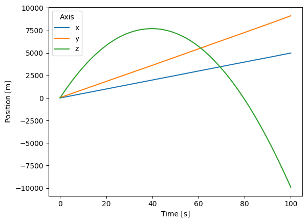
You’ll see that some of the position z values are negative. We know that this doesn’t make much sense since z values of 0.0 correspond to ground-level.

In fact, what would make most sense would be to end the simulation once the projectile reaches a z value of 0.

pos_above_z_0 = simulation.position.where(simulation.position.sel(ax="z") < 0)
simulation = simulation.where(pos_above_z_0, drop=True)

simulation.position.plot(hue="ax")
plt.show()

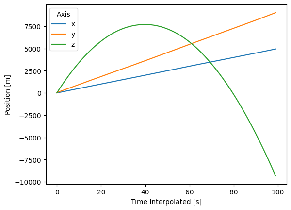
Interpolating the position at any time

Now we have the position of the projectile at the time points for which our onboard sensors have recordings. However, these time points are full of noise. What if we want to clean this up a little and find the position only at certain times? We can use xarray’s interpolation capabilities!

time_max = simulation.time.max()

time_interp_values = np.arange(0, time_max)

simulation_interp = simulation.interp(time=time_interp_values)

simulation_interp.time.attrs["long_name"] = "Time Interpolated"
simulation_interp.time.attrs["units"] = "s"

simulation_interp.position.plot(hue="ax")
plt.show()

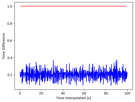
Take a look at how our new times are linearly spaced as opposed to the original simulation’s time values.

simulation.time.diff(dim="time").plot(c="blue")
simulation_interp.time.diff(dim="time").plot(c="red")
plt.ylabel("Time Difference")
plt.show()

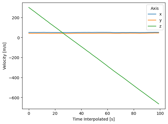
And, note that we have interpolated the entire simulation! That means that not only is our position interpolated, but so is our acceleration, and velocity!

simulation_interp.velocity.plot(hue="ax")

[<matplotlib.lines.Line2D at 0x7f900b1a8ce0>,
 <matplotlib.lines.Line2D at 0x7f900b1a8d10>,
 <matplotlib.lines.Line2D at 0x7f900b1a8dd0>]

Conclusion

It’s about time to wrap this up. Hopefully you’ve seen that you can do some really cool stuff with xarray, and that API is really expressive. This is not an exhaustive tutorial, but hopefully will inspire you to consider using xarray for you next modeling and simulation task!