Best Wordle Words

Wordle is extremely popular these days, and for good reason: it is so simple and elegant; a real joy.

Wordle reminds us that the best of games are simple in nature, with few rules, and a great deal of freedom for players to develop their own strategies. But, don’t let Wordle’s apparent simplicity fool you… it is all too easy to guess words ineffectively, and to lose!

In this arrticle I will try to come up with some good words for initial guesses to Wordle.

5-Letter Words

Let’s assume that the only rule to Wordle’s choice of words is that it is a 5-letter word. So, let’s just get all 5-letter words.

import string

import matplotlib.pyplot as plt
import pandas as pd
import requests


def plot_table(df: pd.DataFrame):
    return df.style.background_gradient("YlGn")


words_request = requests.get(
    "https://gist.githubusercontent.com/nicobako/759adb8f0e7fa514f408afb946e80042/raw/d9783627c731268fb2935a731a618aa8e95cf465/words"
)
all_words = words_request.content.decode("utf-8").lower().split()

five_letter_words = pd.DataFrame(
    (
        word
        for word in all_words
        if len(word) == 5 and all(letter in string.ascii_lowercase for letter in word)
    ),
    columns=["word"],
)

How many 5-letter words do we have?

len(five_letter_words)

6071

Wow! That’s a lot!

Criteria for a Good Guess

There are many theories on what makes a good guess, so please don’t judge… but here is my naive simple criteria for a good guess:

• Contains as many common letters as possible

• Contains as many different letters as possible

• Contains as many letters in common places as possible

For now, let’s keep it this simple. We can always make things more complicated later…

Collecting the Data

This is not so tricky… We look at each word, look at which letters we find at each position in each word, and keep track of everything. Later we can use this data to calculate everything we need.

def get_letters_data():
    data = []
    for word in five_letter_words["word"]:
        for position, letter in enumerate(word):
            data.append({"letter": letter, "position": position + 1})
    return pd.DataFrame(data)


letters = get_letters_data()

This data is a table whose rows contain two values: a letter; its position in a word. It might not seem like much, but it’s all we need. Here’s a quick glance at what this table looks like:

letters.head()

	letter	position
0	a	1
1	a	2
2	r	3
3	o	4
4	n	5

Most Common Letters

Given our data, we can now count the occurences of each letter. This reflects how commonly each letter is found in any word. To calculate this we take a look at our letters data, group them by letter, and tally up the count.

letters_count = letters.groupby("letter").count()
letters_count.columns = ["count"]
letters_count = letters_count.sort_values(by="count", ascending=False)
letters_count.plot.barh(y="count")
plt.show()

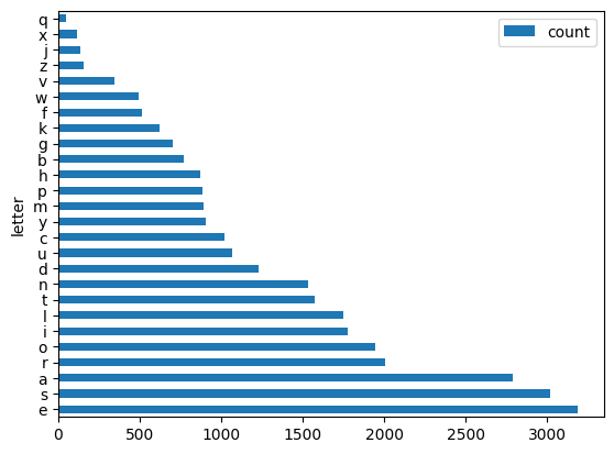
I don’t know about you, but these results surprised me! The top 10 letters are:

plot_table(letters_count.head(10))

	count
letter
e	3187
s	3019
a	2785
r	2006
o	1946
i	1776
l	1746
t	1574
n	1535
d	1232

And the lowest 10 are:

plot_table(letters_count.tail(10))

	count
letter
b	768
g	704
k	620
f	514
w	494
v	343
z	160
j	136
x	117
q	49

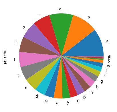
Let’s create a new column in our letters-count table with the percent occurence of each letter:

letters_count["percent"] = 100 * letters_count["count"] / letters_count["count"].sum()

As usual, the sum of the percent column should equal 100%.

letters_count["percent"].sum()

100.0

letters_count["percent"].plot.pie(y="letter")
plt.show()

Words With Most Common Letters

Using the occurence of each letter, we can look at all of our words, and give them a score based on how common the letters of the word are.

We also don’t want to give words extra points for having the same letter multiple times… Remember, the whole point of this is to come up with a good first guess for Wordle, so it would be more helpful if our first guess contained unique letters.

def score_based_on_letters_count(word: str) -> float:
    score = 0.0
    unique_letters = list(set(word))
    for letter in unique_letters:
        score += letters_count.loc[letter].percent
    return round(score, 2)

In this way, the score of a letter like apple is:

score_based_on_letters_count("apple")

28.34

We can take this metric and calculate a score for all of our 5-letter words.

five_letter_words["score_letters_count"] = [
    score_based_on_letters_count(word) for word in five_letter_words["word"]
]

Let’s take a look at some of the top words:

plot_table(
    five_letter_words.sort_values("score_letters_count", ascending=False)
    .head(10)
    .set_index("word")
)

	score_letters_count
word
arose	42.640000
arise	42.080000
aries	42.080000
raise	42.080000
earls	41.980000
laser	41.980000
reals	41.980000
aloes	41.780000
stare	41.410000
tears	41.410000

Most Common Positions of Letters

Another important thing to look at is the relative position of the letters in our first guess. We want a word whose letters are not only common, but whose positions of letters are in common places.

This is a little trickier to do, but stil not that tough. We group our data by letter and position, and count how many occurences of each letter-position combination.

letters_position = pd.DataFrame(
    {"count": letters.groupby(["letter", "position"]).size()}
)

Here’s what it looks like for the letter a

letters_position.loc["a"]

	count
position
1	338
2	1076
3	646
4	412
5	313

You can see that a is most commonly in the second position.

Let’s create a percent column for this table as well.

letters_position["percent"] = (
    100 * letters_position["count"] / letters_position["count"].sum()
)
letters_position["percent"] = [round(num, 2) for num in letters_position["percent"]]

Let’s make sure the sum of the percent is 100%.

letters_position["percent"].sum()

99.94999999999999

And here’s a fancy chart displaying how the letters and positions look for each letter:

letters_position_pivoted = letters_position.reset_index().pivot(
    index="letter", columns="position", values="percent"
)
letters_position_pivoted.sort_values("letter")
letters_position_pivoted.style.background_gradient("YlGn")

position	1	2	3	4	5
letter
a	1.110000	3.540000	2.130000	1.360000	1.030000
b	1.480000	0.130000	0.510000	0.340000	0.070000
c	1.520000	0.260000	0.600000	0.850000	0.140000
d	1.070000	0.190000	0.660000	0.780000	1.350000
e	0.580000	2.410000	1.290000	3.980000	2.240000
f	0.990000	0.040000	0.230000	0.290000	0.130000
g	0.930000	0.070000	0.530000	0.580000	0.200000
h	0.830000	0.910000	0.130000	0.250000	0.740000
i	0.290000	2.210000	1.850000	1.210000	0.300000
j	0.380000	0.010000	0.040000	0.020000	nan
k	0.360000	0.100000	0.310000	0.760000	0.510000
l	0.970000	1.290000	1.430000	1.250000	0.810000
m	1.130000	0.250000	0.720000	0.600000	0.240000
n	0.440000	0.510000	1.530000	1.410000	1.160000
o	0.360000	2.980000	1.570000	1.030000	0.480000
p	1.240000	0.350000	0.490000	0.570000	0.270000
q	0.120000	0.030000	0.010000	0.000000	nan
r	0.900000	1.630000	1.810000	1.110000	1.160000
s	2.500000	0.180000	0.840000	0.870000	5.560000
t	1.240000	0.420000	0.900000	1.470000	1.160000
u	0.180000	1.690000	1.020000	0.540000	0.080000
v	0.370000	0.110000	0.420000	0.220000	0.010000
w	0.750000	0.250000	0.310000	0.220000	0.090000
x	0.020000	0.080000	0.190000	0.010000	0.090000
y	0.150000	0.310000	0.290000	0.140000	2.080000
z	0.080000	0.040000	0.180000	0.130000	0.090000

This chart is really quite useful, from a glance you can see that some letters are much more likely to be in certain positions of the word, so when making guesses, it’s important to keep this in mind.

Words with Most Common Letter Positions

We can use the above data to score each of our 5-letter words based on the positions of the letters. We just look at all of the letters of our word and their corresponding positions, and tally up the percent chance of encountering each letter in its position.

Here will count all letters, even duplicates… not sure why, it just feels right.

def score_based_on_letters_position(word: str) -> float:
    score = 0.0
    for i, letter in enumerate(word):
        position = i + 1
        score += letters_position.loc[letter, position]["percent"]
    return score

So, the score of apple in this case would be:

score_based_on_letters_position("apple")

5.44

You can see right away that the score for the word apple is very different than before.

Let’s calculate the score for each of our 5-letter words based on the positions of its letters.

five_letter_words["score_letters_position"] = [
    score_based_on_letters_position(word) for word in five_letter_words["word"]
]

Let’s take a look at the top 10 in this case.

plot_table(
    five_letter_words[["word", "score_letters_position"]]
    .sort_values("score_letters_position", ascending=False)
    .head(10)
    .set_index("word")
)

	score_letters_position
word
sales	17.010000
sores	16.830000
sates	16.480000
soles	16.450000
cares	16.410000
bares	16.370000
sames	16.300000
sades	16.240000
tares	16.130000
pares	16.130000

You may be surprised, as I was, to find that these two ways of scoring words generated very different lists!

What is the Best Guess?

So, what is the best first guess. We’ll naively assume that is a combination of these two scoring methods. We’ll just add up the scores for letter-count and letter-position, and look at the top words.

five_letter_words["final_score"] = (
    five_letter_words["score_letters_count"]
    + five_letter_words["score_letters_position"]
)

plot_table(
    five_letter_words.sort_values("final_score", ascending=False)
    .set_index("word")
    .head(20)
)

	score_letters_count	score_letters_position	final_score
word
tares	41.410000	16.130000	57.540000
tales	40.560000	15.750000	56.310000
rates	41.410000	14.880000	56.290000
dares	40.290000	15.960000	56.250000
aries	42.080000	14.130000	56.210000
cares	39.600000	16.410000	56.010000
lanes	40.430000	15.580000	56.010000
oates	41.220000	14.340000	55.560000
aloes	41.780000	13.510000	55.290000
pares	39.140000	16.130000	55.270000
mares	39.170000	16.020000	55.190000
bares	38.760000	16.370000	55.130000
dales	39.430000	15.580000	55.010000
hares	39.100000	15.720000	54.820000
earls	41.980000	12.740000	54.720000
danes	38.730000	15.680000	54.410000
reals	41.980000	12.250000	54.230000
earns	41.280000	12.900000	54.180000
races	39.600000	14.580000	54.180000
canes	38.050000	16.130000	54.180000

Conclusion

Don’t let this fancy code and math fool you, this is a naive approach. We are simply looking at which letters are most common, and which positions of letters are most common, and picking words that maximize this combination. There are a ton of other details that this code simply isn’t considering, and a lot of ways this code can be improved.

In the end, this article may help you come up with a decent first guess, but the rest is up to you! Anyway, good luck on your next Wordle game, and don’t forget to try out one of the top words!